Let random variable X ∼ Pareto(a, b) with pdf f(x):
In[1]:= ![]()
and let random variable Y ∼ Uniform(α, β) with pdf g(y):
In[2]:= ![]()
Problem: Find the pdf of V = X Y, denoted h(v).
Solution: The solution is simply:
In3]:= ![]()
Out[3]= 
A quick Monte Carlo ‘check’ of the exact solution we have just derived:
It is always a good idea to check that a theoretical solution that has been derived is consistent with pseudo-random data. To illustrate, let us suppose that (a=2, b=3, α=1, β=4). To perform a quick Monte Carlo check, we first generate 100000 pseudo-random drawings of X, and 100000 pseudo-random drawings of Y:
In[4]:= ![]()
We now make a frequency plot of the product of the X and Y pseudo-random data, and then compare the pseudo-random Monte Carlo solution (—) with the theoretical symbolic solution h(v) (—) derived above:
In[5]:= ![]()
Out5= 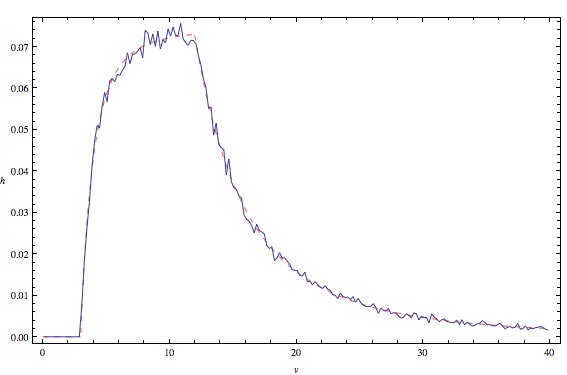
Looks good!
Let random variable X ∼ N(0,1) with pdf f(x):
In[1]:= 
The pdf of the product of two standardised Normals can then be elegantly derived via:
In[2]:= ![]()
Out[2]= 
Let random variable X ∼ Triangular(-1/2, 1, 2) with pdf f(x):
In[1]= 
and let random variable Y ∼ Triangular(-1, 2, 3) with pdf g(y):
In[2]= 
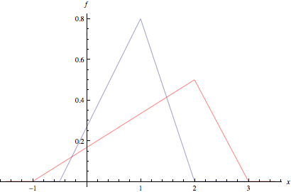
The following diagram plots the pdf of both f(x) (—) and g(y) (—):
Problem: Find the pdf of V = X*Y (i.e. the pdf of the product of the two random variables).
Solution: Here is the solution pdf, say h(v):
In[3]:= ![]()
Out[3]= 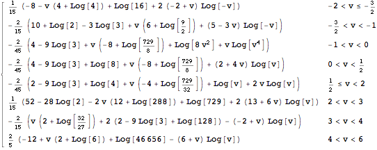
In[4]:= ![]()
The solution has a piecewise form. Here is a plot of the solution pdf:
In[5]:= ![]()
Out[5]= 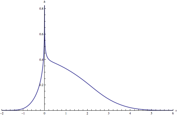
A quick Monte Carlo ‘check’ of the exact solution we have just plotted:
It is always a good idea to check that a theoretical solution that has been derived is consistent with pseudo-random data. Here, we generate 100000 pseudo-random drawings of X and 100000 pseudo-random drawings of Y:
In[7]:= 
We can now make a frequency plot of the product of the X and Y pseudo-random data, and then compare the pseudo-random Monte Carlo solution (—) with the theoretical symbolic solution h(v) (—) derived above:
In[8]:= ![]()
Out[8]= 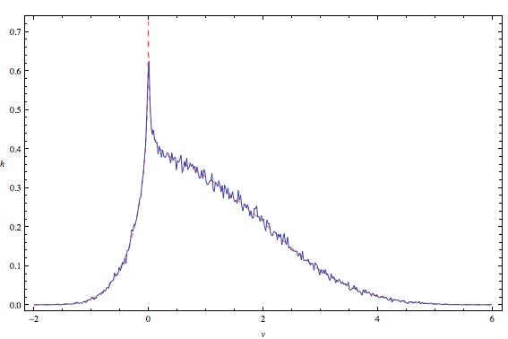
For the win!